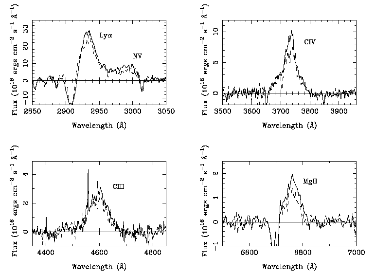
Old Q0957+561 data & software:
![]()
![]()
![]()

► Simple FORTRAN programs to apply the d2 test (accurate and robust time delay measurements)
► Photos
Advertising:
Introduction to GL
![]()
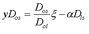
(ii) The
lens equation
It is necessary to study the
physics of lensing for understand the GL events. In the simplest situation,
we will have a source located at S, while the observer sits at O. The lens
(the simplest one is a point mass, or “Schwarzschild lens”) is located at
a distance
![]() from O, on the optic axis.
from O, on the optic axis.
![]() and
and
![]() are the angular-diameter distances between
lens and source plane and observer and source plane, respectively (see figure 5). It is important to note that angular-diameter
distances are not euclidean distances, so in general:
are the angular-diameter distances between
lens and source plane and observer and source plane, respectively (see figure 5). It is important to note that angular-diameter
distances are not euclidean distances, so in general:
![]() , because of Einstein’s universe is not flat.
, because of Einstein’s universe is not flat.
|
|
|
figure 5: Typical
lensing configuration for a point mass lens. The source is located
at the position S, while the observer sits at O. The lens is located
in a plane a distance
|
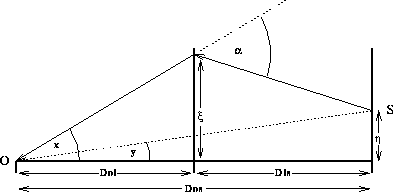
A ligth ray which passes the lens (with mass
![]() ) at a distance
) at a distance
![]() is deflected by
is deflected by
![]() , the deflection angle given by equation [3] (note that
, the deflection angle given by equation [3] (note that
![]() ). From simple geometry, we can obtain the condition for this ray to reach
the observer at O:
). From simple geometry, we can obtain the condition for this ray to reach
the observer at O:
 [4]
[4]
The angular separation
between the deflecting mass and the deflected ray is:
 [5]
[5]
hence, from equation
[4]:
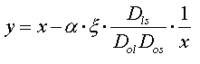
From equation [3] (here
![]() ), we can rewrite this equation:
), we can rewrite this equation:
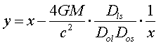 [7]
[7]
Rearranging this equation:
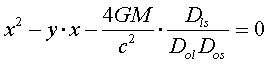 [8]
[8]
Solving this equation
we obtain:
 [9b]
[9b]
which are the two solutions
(a,b) for the second degree equation [8].
The angular separation between the images a and b is:
 [10]
[10]
and the angular separation
between the source and the lens is related to the image positions by:
![]() [11]
[11]
The ray-trace equation
[8] always has two solutions of opposite sign.
This means that the source has an image on each side of the lens.
If source, lens and observer
are colinear then a special situation arises. We will have an “Einstein
Ring”, because of there is circular symmetry. In that case we have the
mathematical condition:
![]() [12]
[12]
Hence, the image solutions
([9a], [9b]) are (see figure 6):
 [13a]
[13a]
 [13b]
[13b]
|
figure 6:
When source, lens and observer are colinear, there is circular symmetry,
and we can observe an “Einstein Ring”. |
We can now define the
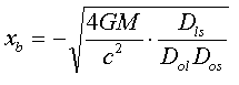
“Einstein Radius”, like the radius of the “Einstein Ring”:
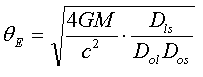 [14]
[14]
Now we find a problem: the description of a lens like a point
mass is not enough realistic in most situations, because the “Schwarzschild
lens” is an idealization. We need to develop a mathematical formalism and
find a lens equation suitable to all mass distributions. When
we study more general situations, we cannot suppose that the lens
is circular-symmetric, so we have to see the angular separations, the impact
parameter and the angles involved in the formalism like two dimensional vectors
projected onto the lens or source plane. The geometry in the GL event with
a general mass distribution is similar to the point mass one, so we can obtain
a equation similar to [6], but with vectorial terms:
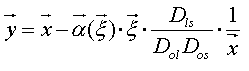 [15]
[15]
Because the angles involved
in GL events are very small, it is evident, from elemental geometry (see
figure 5), that:
 [16]
[16]
hence:
 [17]
[17]
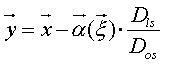
Or, in terms of the distance
![]() (see figure 5) from the
source to the optical axis:
(see figure 5) from the
source to the optical axis:
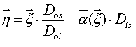
Given the matter distribution of the
lens and the position
![]() of the source, the equation
[18] may have more than one solution
of the source, the equation
[18] may have more than one solution
![]() . This means that the same source can be seen at several positions at the
sky.
. This means that the same source can be seen at several positions at the
sky.
Now we have another problem:
to know the deflection law
![]() . For geometrically-thin lenses (we can reject the width of the lens
in the optical axis, projecting all the mass of the lens onto the lens plane,
if we compare it to the huge distances involved in the GL event) the deflection
angles of several point masses simply add [SCH92]. Hence
we can descompose a general matter distribution into small parcels of mass
mi and write the deflection angle as:
. For geometrically-thin lenses (we can reject the width of the lens
in the optical axis, projecting all the mass of the lens onto the lens plane,
if we compare it to the huge distances involved in the GL event) the deflection
angles of several point masses simply add [SCH92]. Hence
we can descompose a general matter distribution into small parcels of mass
mi and write the deflection angle as:
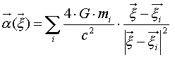 [19]
[19]
where
![]() describes the position of the ligth ray in the
lens plane, and
describes the position of the ligth ray in the
lens plane, and
![]() describes the position of the point mass mi
in the same plane. We can take the continuum limit and find:
describes the position of the point mass mi
in the same plane. We can take the continuum limit and find:
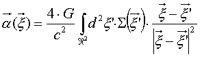 [20]
[20]
where we have defined:
![]() [21]
[21]
where
![]() is the surface element of the lens plane, and
is the surface element of the lens plane, and
![]() is the surface mass density at position
is the surface mass density at position
![]() which results if the volume mass distribution
of the deflector is projected onto the lens plane.
which results if the volume mass distribution
of the deflector is projected onto the lens plane.
![]()
Click on the arrow below to return to the previous page.
![]()