Old Q0957+561 data & software:
![]()
![]()
![]()

► Simple FORTRAN programs to apply the d2 test (accurate and robust time delay measurements)
► Photos
Advertising:
|
d2
TEST:
SOME SIMPLE FORTRAN
PROGRAMS
|
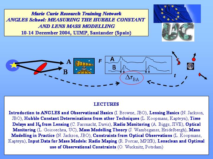
What is the d2 test?
We can accurately and robustly measure the time delay between the
intrinsic features that appear in two images A and B of a multiple QSO (with
relation to A, we assume that B is delayed in TBA). As it was discussed by
Lehar et al. (1992, ApJ 384, 453), the irregular delay-peak of the AB
cross-correlation function should be closely traced by the symmetrical
central peak (around the lag t = 0) of the
AA (or BB) autocorrelation function. Moreover, other features of
the cross-correlation function around lags t1,
t2,... will be closely reproduced in
the autocorrelation function around lags t1-TBA,
t2-TBA,...,
respectively. Therefore, if the shifted discrete autocorrelation
(DAC) is matched to the discrete cross-correlation (DCC), in
principle, one derives an
accurate
and robust value
of the time delay. This self-consistent methodology is called the
delta-square test, and it was successfully applied to some golden
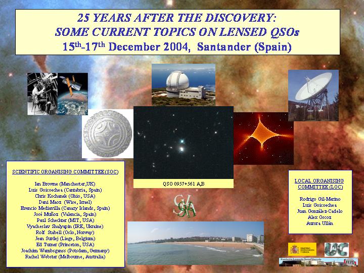
datasets for QSO 0957+561 (e.g., Goicoechea et al. 1998, Ap&SS 261, 341;
Serra-Ricart et al. 1999, ApJ 526, 40). The technique belongs to a "second
generation" of methodologies to infer time delays, since it only works
when one knows a rough value of the delay. The rough estimation T may be
done from a simpler technique ("first generation"). Before to apply the
d2 test, we need to make a
golden dataset.
A golden dataset contains an ACTIVE and FREE FROM LONG GAPS
light curve A during a period [ti,tf]
and an ACTIVE and FREE FROM LONG GAPS light curve B
during a period [ti + T,tf + T]. It is also
required the HOMOGENEOUS MONITORING of both images. In some cases (if
there are microlensing events, observational problems,...), the intrinsic
variability is corrupted and important distortions in the features of the
cross-correlation function appear as compared with the corresponding
features in the autocorrelation functions. Therefore, as a final analysis,
we must compare the AA (or BB) autocorrelation and the AB cross-correlation.
IF THERE ARE NO IMPORTANT DIFFERENCES BETWEEN AA (OR BB) AND AB,
then all is ok and we can apply the technique. While some "first
generation" methods give delays mainly based on the dominant features of
the light curves, our methodology is sensitive to the whole information.
Do you want to play with d2?
We invite you to use the Q0957+561A, B data by Kundic et al. You may take the main event in A-1995 (95P.DAT) and the main event in B-1996 (96P.DAT), or alternatively, the secondary event in A-1995 (95S.DAT) and the secondary event in B-1996 (96S.DAT). For the main events, cross-correlations and autocorrelations are described in CROSP.FOR (outputs: CROSP5.DAT and CROSP15.DAT) and AUTOP.FOR (outputs: AUTOP5.DAT and AUTOP15.DAT). For the secondary events: CROSS.FOR (CROSS5.DAT, CROSS15.DAT), AUTOS.FOR (AUTOS5.DAT, AUTOS15.DAT). In order to compare AA and AB, one could use ACCP5FIG.FOR/ACCP15FIG.FOR (main) or/and ACCS5FIG.FOR/ACCS15FIG.FOR (secondary). Are you ready to apply the test?. The d2 technique appears in DELTAP.FOR (outputs: DELTAP5.DAT, DELTAP15.DAT) and DELTAS.FOR (outputs: DELTAS5.DAT, DELTAS15.DAT) for the main and secondary events, respectively....and the errors?. The programs to derive errors are: (1) ERRORP5SIM.FOR (output: ERRORP5SIM.DAT) for the main events, and (2) ERRORS5SIM.FOR (output: ERRORS5SIM.DAT) for the secondary events. A comparison of results (main events vs. secondary events) is really instructive.