Old Q0957+561 data & software:
► Simple FORTRAN programs to apply the d2 test (accurate and robust time delay measurements)
► Photos
Advertising:
|
GLITP / OPTICAL MONITORING OF QSO 0957+561 |
The Gravitational Lenses International Time Project (GLITP) collaboration observed the first gravitational lens system (QSO 0957+561) from 2000 February to 2000 March 31. The daily VR observations were made with the 2.56-m Nordic Optical Telescope at Roque de los Muchachos Observatory, La Palma (Spain). We have derived detailed and robust VR light curves of the two components Q0957+561A and Q0957+561B (empirical-PSF photometry, V, R).
At an initial stage, we found "surprising" daily variabilities, which were similar in both components. The figure include these daily or residual
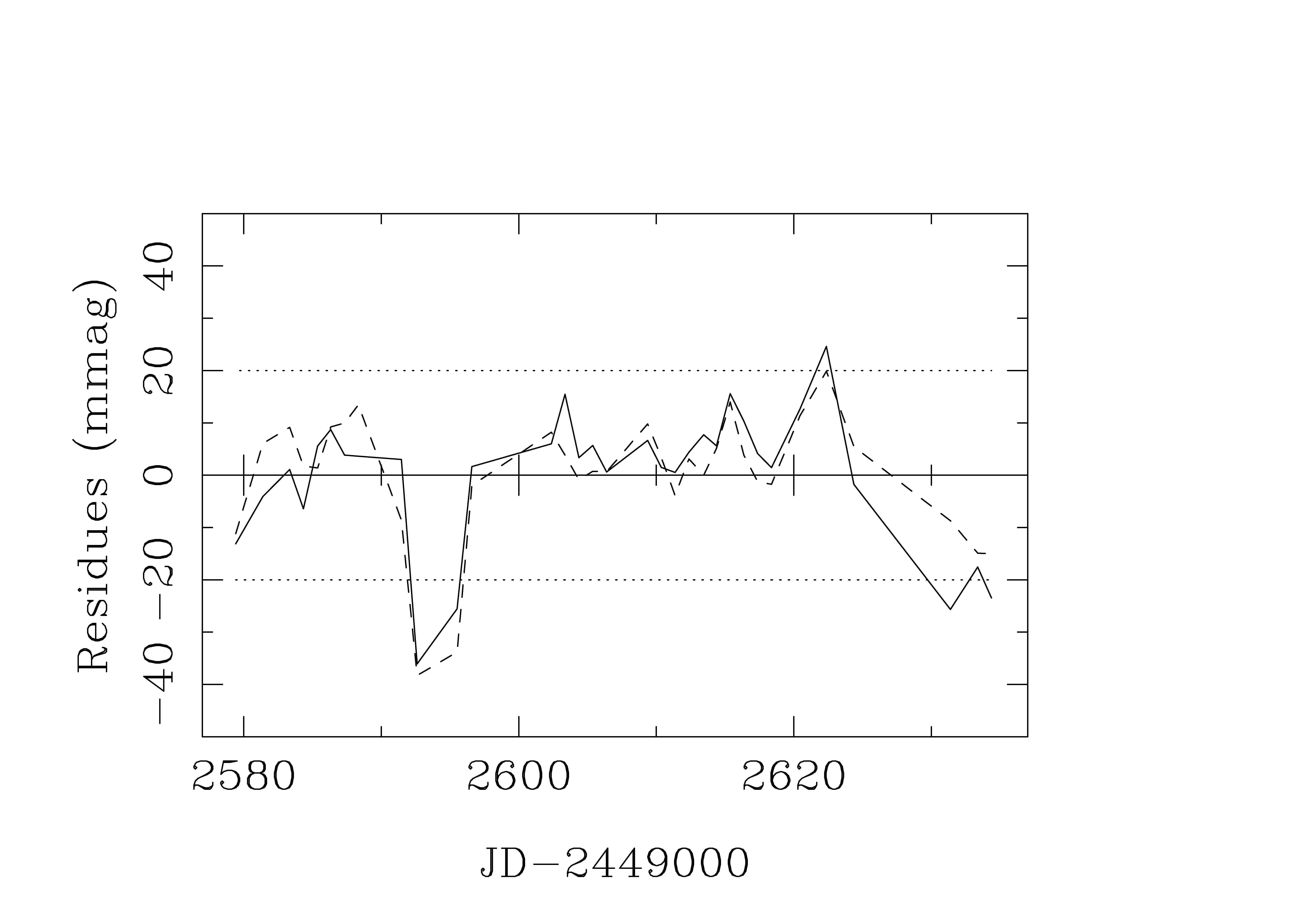
(superimposed to linear gradients) signals in the R band. The prominent peaks in the signals correspond to images that lead to "rare" physical parameters of the lens galaxy. The photometric method is not able to accurately extract the galaxy information, so it seems reasonable to find a peak of noise in the measurement of other quantities, e.g., the QSO fluxes. What is the reason for the peaks of observational systematic noise?. First, the PSF may vary over the field because of the optics of the telescope and camera, and the variation may be more significant in good seeing conditions (most of the peaks are associated with good seeing conditions). Alternatively, as a second possibility, the effective PSF associated with each object could depend on the object flux and other factors, so the stellar PSFs would be different to the PSF of the components. In other words, a slight mismatch between the reference PSF and the PSF in the lens system region could be responsible for the peaks of noise. Some level of systematic noise may also appear from other photometric techniques, e.g., aperture photometry. Apart from excellent seeing conditions, through a direct aperture photometry, one cannot avoid a similar leakage of signal in both apertures as well as a similar cross-contamination of the QSO fluxes. Using a correction law depending on seeing, a systematic perturbation could be present yet. For example (in our PSF scheme), after subtracting the background, if we analyze a R-band image leading to small noise (2000 March 12), we obtain the figures:
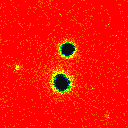
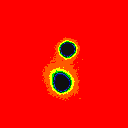
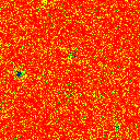
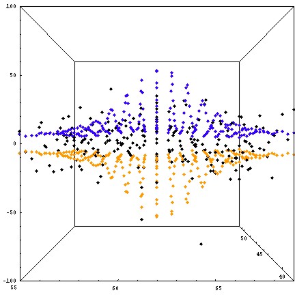
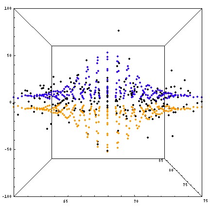
While the group of three color images represents: the original frame (left), a model frame (centre) and the residual (real -mod) frame (right), the other two 3D figures show the residual counts (black diamonds) and rough Poisson fluctuations (± N1/2) for the two components A and B. This day all seem to be ok. However, if we analyze the R-band image corresponding to the maximum noiseto small noise (2000 February 18), the conclusion is quite different. One infers new figures:
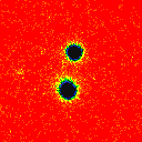
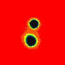
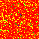
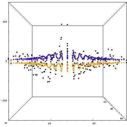
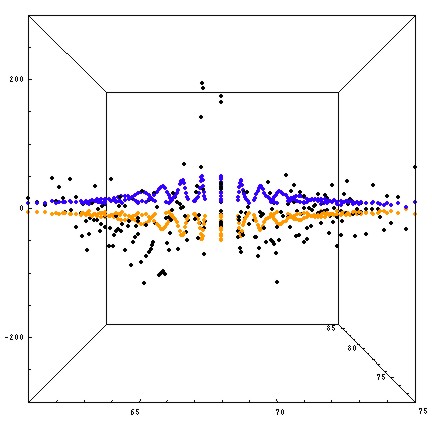
In the new original (real) frame/model frame/residual frame picture are not clear evidences for an anomaly. However, the 3D figures (counts vs. 2D pixel position) show a similar anomaly in both components. In different regions, the residual counts clearly exceed the rough Poissonian fluctuations, and moreover, there is an evident bias between the real trends and the modeled ones: excesses in the centres and a lacks in the tails. The bias is consistent with components that are modeled from a relatively broad stellar profile (PSF). In order to get an accurate photometry, at the final stage, the observational noise peaks were dropped.
The directory contains 77 frames in FITS format (GZ compressed, about 3.2 Mb/frame). Each frame has a label that includes: (a) date (e.g., "00Feb8" = 2000 February 8), (b) optical filter (e.g., "V" = V-band), (c) system ("0957" = QSO 0957+561), and (d) pre-processing step ("f" = final step, which includes bias subtraction and flat-fielding using sky flats). The frames are ready for any photometric task!, good luck!.


